Compass Input Requirement
Please note that the input for Compass should be mRNA's TPM (Transcripts Per Million) expression values, not raw counts or other forms of mRNA expression values. TPM calculation is similar to FPKM but differs in the normalization process. In TPM, all transcripts are normalized for length first. Then, instead of using the total overall read count for size normalization, the sum of the length-normalized transcript values is used as a size indicator.
Please fell free to contact me if you have any questions on this.
Data Processing Recommendation
If your data is in raw sequence format (FASTQ) or as raw counts, we recommend processing it using the following bioinformatics pipeline. This recommendation is based on the fact that our pretrained TCGA (The Cancer Genome Atlas) data was processed using this pipeline, and using the same pipeline for your input data may yield better results.
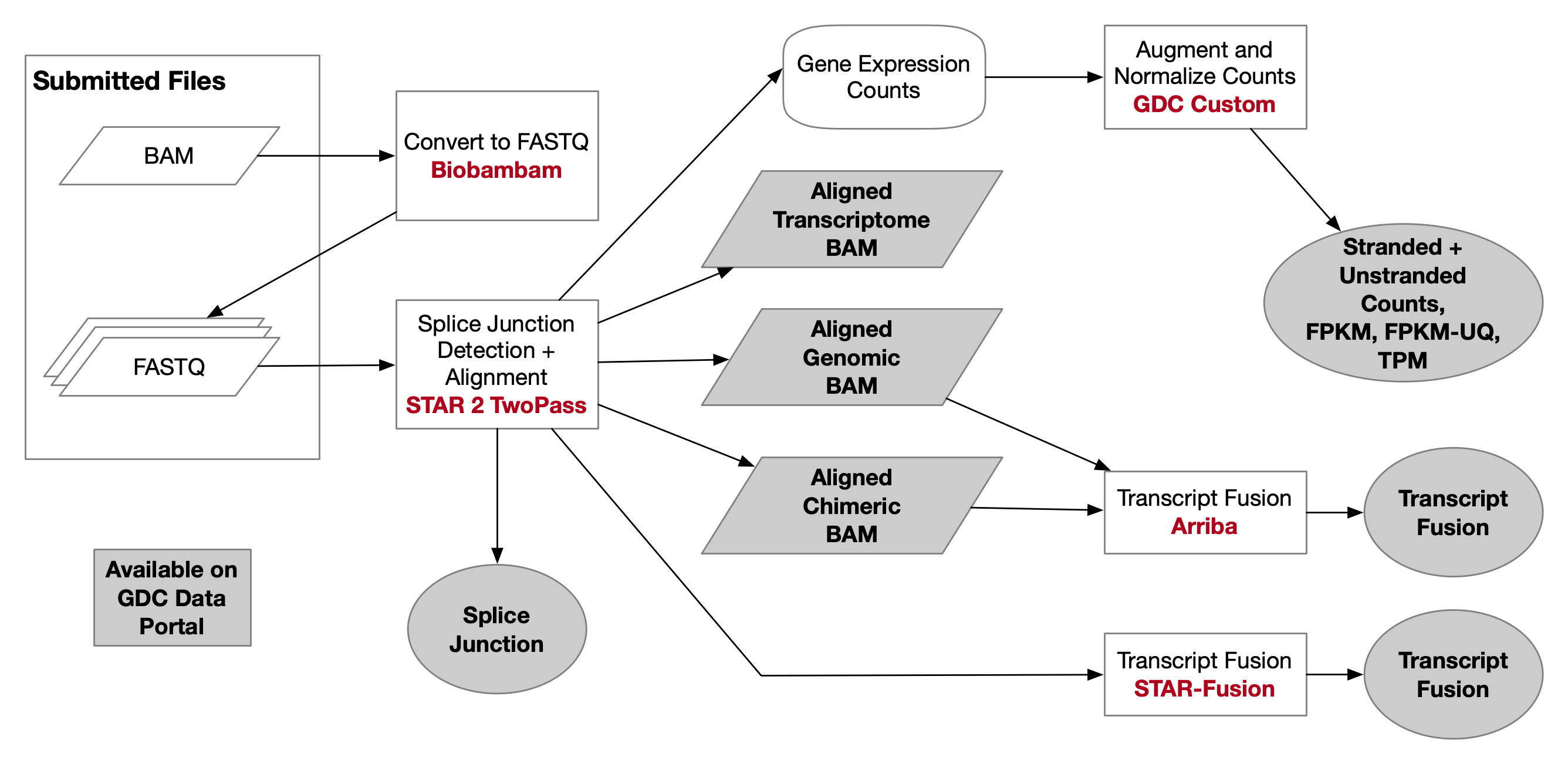
1. mRNA-Seq Alignment Workflow
The RNA-Seq Alignment Workflow follows these steps:
fastqc/multiqc --> fastp ---> STAR2 align (two-pass method)
For more information, please refer to GDC mRNA expression pipeline.
Specific Process
- Begin with quality control using fastqc and multiqc.
- Proceed with data preprocessing using fastp to clean raw sequencing data and improve quality.
- Finally, align the RNA-seq reads to a reference genome using STAR version 2.7.5c, which maps RNA-seq reads to the reference genome. While custom index files can be created, we use the reference genome files downloaded from GDC. The link for the specific reference genome file (star-2.7.5c_GRCh38.d1.vd1_gencode.v36.tgz) is available here.
2. Converting mRNA Raw Counts to TPM
If your data is in mRNA expression counts, you can convert the mRNA raw counts to TPM values using the following method. This process involves normalization using gene lengths, so you will need to download the gene annotation file (v36).on.gtf.gz
Step 1: Download the human GENCODE annotation file (v36)
Download the GENCODE human annotation file (version 36) from the following link:
wget https://ftp.ebi.ac.uk/pub/databases/gencode/Gencode_human/release_36/gencode.v36.annotation.gtf.gz
mv gencode.v36.annotation.gtf.gz ./data
step2: using rnanorm tool to convert Count to TPM
#install rnanorm
pip install rnanorm
from rnanorm import FPKM, TPM, CPM, TMM
gtf_path = "./gencode.v36.annotation.gtf"
tpm = TPM(gtf_path).set_output(transform="pandas")
df_tpm = tpm.fit_transform(df_counts)
step3: Now let's test on an example file
# import packages
import pandas as pd
from rnanorm import FPKM, TPM, CPM, TMM
# convert count to TPM based the gtf file
gtf_path = "https://www.immuno-compass.com/download/other/gencode.v36.annotation.gtf.gz"
tpm = TPM(gtf_path).set_output(transform="pandas")
# example of the raw counts
df_counts = pd.read_csv('https://www.immuno-compass.com/download/other/toy_raw_counts.csv', index_col=0)
df_counts.head()
| ENSG00000223972.5 | ENSG00000227232.5 | ENSG00000278267.1 | ENSG00000243485.5 | ENSG00000284332.1 | ENSG00000237613.2 | ENSG00000268020.3 | ENSG00000240361.2 | ENSG00000186092.6 | ENSG00000238009.6 | ... | ENSG00000198886.2 | ENSG00000210176.1 | ENSG00000210184.1 | ENSG00000210191.1 | ENSG00000198786.2 | ENSG00000198695.2 | ENSG00000210194.1 | ENSG00000198727.2 | ENSG00000210195.2 | ENSG00000210196.2 | |
|---|---|---|---|---|---|---|---|---|---|---|---|---|---|---|---|---|---|---|---|---|---|
| ERR2208944 | 6 | 201 | 0 | 0 | 0 | 1 | 0 | 0 | 0 | 0 | ... | 1376 | 0 | 0 | 0 | 947 | 178 | 0 | 582 | 0 | 4 |
| ERR2208928 | 0 | 222 | 1 | 0 | 0 | 0 | 0 | 0 | 0 | 0 | ... | 2263 | 0 | 0 | 0 | 2549 | 459 | 0 | 1486 | 0 | 0 |
| ERR2208949 | 1 | 487 | 0 | 0 | 0 | 3 | 0 | 0 | 0 | 0 | ... | 2544 | 1 | 0 | 0 | 1783 | 377 | 0 | 745 | 0 | 4 |
| ERR2208900 | 13 | 569 | 0 | 0 | 0 | 14 | 0 | 0 | 0 | 4 | ... | 13168 | 4 | 3 | 1 | 10988 | 2702 | 0 | 3746 | 0 | 101 |
| ERR2208922 | 0 | 29 | 1 | 0 | 0 | 0 | 0 | 0 | 0 | 0 | ... | 14029 | 2 | 0 | 0 | 5480 | 1302 | 0 | 4160 | 0 | 6 |
5 rows × 60660 columns
# example of the TPM values
df_tpm = tpm.fit_transform(df_counts)
df_tpm.to_csv('./toy_tpm.csv')
df_tpm.head()
| ENSG00000223972.5 | ENSG00000227232.5 | ENSG00000278267.1 | ENSG00000243485.5 | ENSG00000284332.1 | ENSG00000237613.2 | ENSG00000268020.3 | ENSG00000240361.2 | ENSG00000186092.6 | ENSG00000238009.6 | ... | ENSG00000198886.2 | ENSG00000210176.1 | ENSG00000210184.1 | ENSG00000210191.1 | ENSG00000198786.2 | ENSG00000198695.2 | ENSG00000210194.1 | ENSG00000198727.2 | ENSG00000210195.2 | ENSG00000210196.2 | |
|---|---|---|---|---|---|---|---|---|---|---|---|---|---|---|---|---|---|---|---|---|---|
| ERR2208944 | 0.460737 | 19.821755 | 0.000000 | 0.0 | 0.0 | 0.109294 | 0.0 | 0.0 | 0.0 | 0.000000 | ... | 133.036440 | 0.000000 | 0.000000 | 0.000000 | 69.629485 | 45.171249 | 0.0 | 67.957710 | 0.0 | 7.837047 |
| ERR2208928 | 0.000000 | 25.382838 | 2.271609 | 0.0 | 0.0 | 0.000000 | 0.0 | 0.0 | 0.0 | 0.000000 | ... | 253.675132 | 0.000000 | 0.000000 | 0.000000 | 217.297235 | 135.050420 | 0.0 | 201.175794 | 0.0 | 0.000000 |
| ERR2208949 | 0.069637 | 43.552412 | 0.000000 | 0.0 | 0.0 | 0.297342 | 0.0 | 0.0 | 0.0 | 0.000000 | ... | 223.052187 | 1.751014 | 0.000000 | 0.000000 | 118.886282 | 86.760220 | 0.0 | 78.887687 | 0.0 | 7.107055 |
| ERR2208900 | 0.172087 | 9.672981 | 0.000000 | 0.0 | 0.0 | 0.263771 | 0.0 | 0.0 | 0.0 | 0.024656 | ... | 219.469413 | 1.331418 | 1.167811 | 0.323478 | 139.272015 | 118.203257 | 0.0 | 75.402463 | 0.0 | 34.112682 |
| ERR2208922 | 0.000000 | 2.360453 | 1.617126 | 0.0 | 0.0 | 0.000000 | 0.0 | 0.0 | 0.0 | 0.000000 | ... | 1119.515705 | 3.187378 | 0.000000 | 0.000000 | 332.563864 | 272.712079 | 0.0 | 400.922453 | 0.0 | 9.702754 |
5 rows × 60660 columns
3. Preparing the inputs for the Compass
The Inputs of Compass model including the cancer type information and TPM values, the genes are identified by gene name, and gene name can be mapped from a dictionary contains the gene Ensembl ID, Entrez gene ID, and gene name.
Please find the cancer code of your data from this table: TCGA Study Abbreviations:
| Study Abbreviation | Study Name |
|---|---|
| LAML | Acute Myeloid Leukemia |
| ACC | Adrenocortical carcinoma |
| BLCA | Bladder Urothelial Carcinoma |
| LGG | Brain Lower Grade Glioma |
| BRCA | Breast invasive carcinoma |
| CESC | Cervical squamous cell carcinoma and endocervical adenocarcinoma |
| CHOL | Cholangiocarcinoma |
| LCML | Chronic Myelogenous Leukemia |
| COAD | Colon adenocarcinoma |
| CNTL | Controls |
| ESCA | Esophageal carcinoma |
| FPPP | FFPE Pilot Phase II |
| GBM | Glioblastoma multiforme |
| HNSC | Head and Neck squamous cell carcinoma |
| KICH | Kidney Chromophobe |
| KIRC | Kidney renal clear cell carcinoma |
| KIRP | Kidney renal papillary cell carcinoma |
| LIHC | Liver hepatocellular carcinoma |
| LUAD | Lung adenocarcinoma |
| LUSC | Lung squamous cell carcinoma |
| DLBC | Lymphoid Neoplasm Diffuse Large B-cell Lymphoma |
| MESO | Mesothelioma |
| MISC | Miscellaneous |
| OV | Ovarian serous cystadenocarcinoma |
| PAAD | Pancreatic adenocarcinoma |
| PCPG | Pheochromocytoma and Paraganglioma |
| PRAD | Prostate adenocarcinoma |
| READ | Rectum adenocarcinoma |
| SARC | Sarcoma |
| SKCM | Skin Cutaneous Melanoma |
| STAD | Stomach adenocarcinoma |
| TGCT | Testicular Germ Cell Tumors |
| THYM | Thymoma |
| THCA | Thyroid carcinoma |
| UCS | Uterine Carcinosarcoma |
| UCEC | Uterine Corpus Endometrial Carcinoma |
| UVM | Uveal Melanoma |
Step1. Add the cancer type information
Suppose your data are all from Melonoma, here is an example to generate the Compass's cancer type
df_cancer_type = pd.DataFrame([], index = df_counts.index)
df_cancer_type['cancer_type'] = 'SKCM'
df_cancer_type.head()
| cancer_type | |
|---|---|
| ERR2208944 | SKCM |
| ERR2208928 | SKCM |
| ERR2208949 | SKCM |
| ERR2208900 | SKCM |
| ERR2208922 | SKCM |
After that, we need to map the cancer type to cancer code:
import json
cancer_code_map = pd.read_json('https://www.immuno-compass.com/download/other/cancer_code.json',
                               orient= 'index')[0]
df_cancer_type['cancer_type'] = df_cancer_type['cancer_type'].map(cancer_code_map)
df_cancer_type.head()
| cancer_type | |
|---|---|
| ERR2208944 | 25 |
| ERR2208928 | 25 |
| ERR2208949 | 25 |
| ERR2208900 | 25 |
| ERR2208922 | 25 |
Step2. Now lets map the df_counts to Compass's input genes.
The dictionary below contains the gene Ensembl ID, Entrez gene ID, and gene name
gene_map = pd.read_csv('https://www.immuno-compass.com/download/other/compass_gene_map.csv')
gene_map.head()
| ensid | gene_name | ensid_v36 | gene_type | gene_supertype | entrezgene | |
|---|---|---|---|---|---|---|
| 0 | ENSG00000121410 | A1BG | ENSG00000121410.12 | protein_coding | protein_coding | 1.0 |
| 1 | ENSG00000148584 | A1CF | ENSG00000148584.15 | protein_coding | protein_coding | 29974.0 |
| 2 | ENSG00000175899 | A2M | ENSG00000175899.15 | protein_coding | protein_coding | 2.0 |
| 3 | ENSG00000166535 | A2ML1 | ENSG00000166535.20 | protein_coding | protein_coding | 144568.0 |
| 4 | ENSG00000128274 | A4GALT | ENSG00000128274.17 | protein_coding | protein_coding | 53947.0 |
df_tpm_input = df_tpm[gene_map.ensid_v36]
df_tpm_input.columns = df_tpm_input.columns.map(gene_map.set_index('ensid_v36').gene_name)
df_tpm_input.shape
(25, 15672)
df_tpm_input.head()
| A1BG | A1CF | A2M | A2ML1 | A4GALT | A4GNT | AAAS | AACS | AADAC | AADAT | ... | ZWILCH | ZWINT | ZXDA | ZXDB | ZXDC | ZYG11A | ZYG11B | ZYX | ZZEF1 | ZZZ3 | |
|---|---|---|---|---|---|---|---|---|---|---|---|---|---|---|---|---|---|---|---|---|---|
| ERR2208944 | 0.000000 | 0.000000 | 859.203620 | 73.019466 | 11.942279 | 1.947147 | 86.527503 | 9.236956 | 3.918524 | 17.763974 | ... | 16.725820 | 14.012390 | 7.255890 | 6.984732 | 16.469669 | 0.879873 | 21.106355 | 89.920944 | 47.520979 | 21.534480 |
| ERR2208928 | 0.038627 | 0.032171 | 881.830260 | 7.533515 | 12.650118 | 2.778540 | 95.158662 | 10.227978 | 1.798357 | 10.818061 | ... | 34.613126 | 42.500215 | 12.806729 | 12.317719 | 18.357604 | 0.526526 | 35.163162 | 60.709750 | 52.413439 | 25.859226 |
| ERR2208949 | 0.030213 | 0.012581 | 504.984491 | 50.836895 | 5.900676 | 0.611231 | 106.174319 | 8.090318 | 4.960132 | 28.557439 | ... | 12.677251 | 19.670726 | 12.836934 | 9.511444 | 9.528438 | 0.154435 | 23.424874 | 69.710920 | 40.638326 | 25.926391 |
| ERR2208900 | 0.143579 | 0.023916 | 1940.416805 | 0.182940 | 4.014771 | 0.813332 | 46.225429 | 2.235265 | 0.042219 | 40.342963 | ... | 24.998045 | 21.527292 | 8.889713 | 7.719297 | 12.813737 | 0.670318 | 18.452489 | 56.563242 | 36.542147 | 32.326600 |
| ERR2208922 | 0.109992 | 0.286277 | 1534.682495 | 0.860539 | 11.887174 | 0.061813 | 83.537696 | 5.875654 | 1.482365 | 16.994521 | ... | 34.388006 | 26.369286 | 3.395453 | 5.485167 | 6.931863 | 0.093706 | 19.792547 | 38.539763 | 25.926938 | 27.002840 |
5 rows × 15672 columns
#### Step3. Generate the inputs and save them
df_inputs = df_cancer_type.join(df_tpm_input)
df_inputs.head()
| cancer_type | A1BG | A1CF | A2M | A2ML1 | A4GALT | A4GNT | AAAS | AACS | AADAC | ... | ZWILCH | ZWINT | ZXDA | ZXDB | ZXDC | ZYG11A | ZYG11B | ZYX | ZZEF1 | ZZZ3 | |
|---|---|---|---|---|---|---|---|---|---|---|---|---|---|---|---|---|---|---|---|---|---|
| ERR2208944 | 25 | 0.000000 | 0.000000 | 859.203620 | 73.019466 | 11.942279 | 1.947147 | 86.527503 | 9.236956 | 3.918524 | ... | 16.725820 | 14.012390 | 7.255890 | 6.984732 | 16.469669 | 0.879873 | 21.106355 | 89.920944 | 47.520979 | 21.534480 |
| ERR2208928 | 25 | 0.038627 | 0.032171 | 881.830260 | 7.533515 | 12.650118 | 2.778540 | 95.158662 | 10.227978 | 1.798357 | ... | 34.613126 | 42.500215 | 12.806729 | 12.317719 | 18.357604 | 0.526526 | 35.163162 | 60.709750 | 52.413439 | 25.859226 |
| ERR2208949 | 25 | 0.030213 | 0.012581 | 504.984491 | 50.836895 | 5.900676 | 0.611231 | 106.174319 | 8.090318 | 4.960132 | ... | 12.677251 | 19.670726 | 12.836934 | 9.511444 | 9.528438 | 0.154435 | 23.424874 | 69.710920 | 40.638326 | 25.926391 |
| ERR2208900 | 25 | 0.143579 | 0.023916 | 1940.416805 | 0.182940 | 4.014771 | 0.813332 | 46.225429 | 2.235265 | 0.042219 | ... | 24.998045 | 21.527292 | 8.889713 | 7.719297 | 12.813737 | 0.670318 | 18.452489 | 56.563242 | 36.542147 | 32.326600 |
| ERR2208922 | 25 | 0.109992 | 0.286277 | 1534.682495 | 0.860539 | 11.887174 | 0.061813 | 83.537696 | 5.875654 | 1.482365 | ... | 34.388006 | 26.369286 | 3.395453 | 5.485167 | 6.931863 | 0.093706 | 19.792547 | 38.539763 | 25.926938 | 27.002840 |
5 rows × 15673 columns
df_inputs.to_csv('./compass_inputs.csv')